Introduction

When dealing with small datasets, leveraging a cloud data warehouse can indeed be a cost-effective choice. However, as your data grows, so do the expenses. This upward cost spiral can be attributed to two main factors

1. Storage and Transfer Costs: Cloud data warehouses charges for storing data in its tables, importing and exporting data into them. Various teams tend to create different datasets and replicate data which leads to higher storage costs.

2. Query Processing Costs: As your dataset grows, queries may need to process more data to generate results, leading to higher processing costs. Writing inefficient and un-necessary queries and poor data modelling practices further increases processing costs.

How to control cost while having the benefits of cloud data warehousing?

Data lakehouse technology provides features to access the data from your cloud storage without moving and replicating the data multiple times and uses distributed framework to keep the cost lower as data scale. In this project, we are focusing on databricks - a data lakehouse that is a all in one platform for your data needs

Here's how Databricks specifically delivers cost savings:

1. Databricks provides a managed Spark environment that allows users to choose the instance types and sizes based on your specific workload requirements, which can help optimize costs

2. It offers flexibility and customization of Spark for ETL use cases. It gives you many parameters to optimize and fine tune your workloads

Databricks vs Bigquery : Hands-on

We did a project to assess the cost-effectiveness of Databricks in comparison to BigQuery.

Data Loading and Creating Table

💡 Dataset Info: We are using a public dataset available in BigQuery marketplace called GDELT 2.0 Event Database.

Tables: We are using a table named iaradio_2grams.
Size in CSV : 1.61 Tib 
Size in Parquet : 85.16 Gib
Rows : 13.16 Billion

The below BigQuery SQL query constructs a new table named project_id.bucket.iaradio_2grams. The data originates from the gdelt-bq.gdeltv2.iaradio_2grams table. Interestingly, it generates a random export_id between 0 and 63 for each record. Additionally, it renames some of the selected columns for better clarity.

To optimize data retrieval, the query partitions the table based on the newly created export_id column, dividing it into 512 segments. This allows for faster searches when filtering by export_id. Finally, the query clusters the table by the same export_id column, potentially enhancing the performance of specific queries, particularly those involving aggregations on this field.

• Creating a seperate with row_number for correctly querying billion rows

-- Creating a seperate with row_number for correctly querying billion rows 
  
CREATE TABLE `project_id.dataset_id.table_id` 
PARTITION BY RANGE_BUCKET(export_id, GENERATE_ARRAY(0, 512, 1)
CLUSTER BY export_id
 AS (
SELECT
  CAST(FLOOR(64*RAND()) AS INT64) AS export_id,
  TIMESTAMP AS time_field,
  DATE AS date_field,
  STATION AS station,
  HOUR AS hour_field,
  NGRAM AS ngram,
  COUNT AS count_field,
  SHOW as show,
FROM

• Export example for each billion

-- Export example for each billion 
  
EXPORT DATA 
  OPTIONS( 
    uri='gs://iaradio/iaradio_2grams/iaradio_2grams-*.parquet',
    format='PARQUET',
    overwrite=true) 
  AS SELECT 
    time_field, date_field, station, hour_field, ngram, count_field
    EXCEPT(export_id)
  FROM

• 💡Result : Successfully exported 13160610182 rows into 1749 files.

💡 Optimisation Tips:

Export the data in different parts for Optimization in Databricks: 

A. If you load all data at once and then read it in databricks. 
 It takes approx 3 hrs to read the data. Overall time 6 hrs

B. If you load all data at once and then read it in parts.Each part of 10 Million rows
takes 1 hr to get converted into delta format. Overall time 13 hrs+  

C. If you load data in parts of 1 billion. So while ready data in databricks and 
converting it in delta format takes 15 mins per query. So Overall time taken is 3.5 hrs

Time saved using option C is 50%.
You reduce loading time even more with some more code optmisations,
whe have talked about it in this blog

Databricks Workspace Creation

1. First Activate your Databricks Trial account :

• It takes 5 mins to do that , create Databricks account.

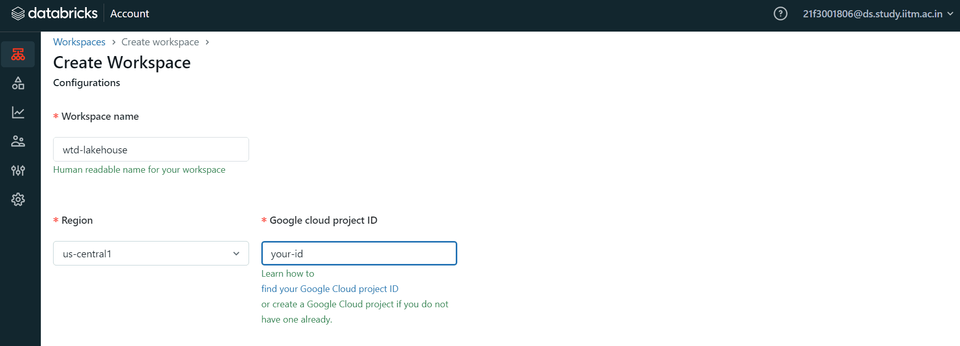
2. Create a new Workspace like this :

• Provide the following details:

  1. Workspace name

  2. Region

  3. Google cloud project_id

  4. We don’t need to set up any advanced configurations.

While Databricks offers a fantastic platform for data exploration and manipulation, understanding what happens behind the scenes during workspace creation can empower you to make informed decisions for cost optimization. Let's dissect the resource provisioning process and explore potential areas for cost control.

GCP Buckets: Essential But Not Free

Databricks creates three GCP buckets upon workspace creation:

• External DBFS Storage: This bucket stores your data. While storage costs are typically the most significant expense, selecting the right storage class based on your data access frequency can lead to significant savings.

• Databricks Logs: Analyzing these logs is crucial, but consider setting up lifecycle management rules to automatically archive older logs to cost-effective storage classes like Nearline Storage.

• Unity Catalog Bucket (if applicable): Similar to Databricks logs, explore lifecycle management for Unity Catalog metadata to optimize storage costs.

Kubernetes Cluster: Power at a Price

The automatically provisioned Kubernetes cluster fuels your data processing needs. However, cluster size and instance types directly impact costs. Utilize tools like cluster autoscaling to ensure you have the necessary compute power while avoiding overprovisioning during idle periods. Consider spot instances for cost-effective compute resources when job runtimes are flexible.

By understanding the resources provisioned during Databricks workspace creation and implementing cost-optimization strategies for GCP buckets and the Kubernetes cluster, you can ensure your data exploration efforts are powerful and budget-friendly.

3. Starting A Compute Cluster

Choosing the right cluster type optimizes both performance and efficiency.

Finding Your Cluster Match:

• All-Purpose Clusters: These versatile workhorses are perfect for interactive exploration, building notebooks, and iterative workflows. They offer a good balance of power and affordability, making them ideal for data lakehouse development.

• Job Clusters: Need to run a long-running job once? These cost-effective clusters spin up, execute the job, and then shut down, saving you money during downtime.

• SQL Warehouse Clusters: Optimized for large-scale SQL queries, these clusters deliver consistent performance for data warehousing tasks.

Right-Sizing Your Cluster:

For personal use and trials, a 32GB memory, 4-core Personal Compute Cluster is a good starting point. But remember, flexibility is key:

• Basic Tasks? A 16GB, 2-core cluster can handle smaller datasets (up to 50GB) efficiently.

• Data-Intensive Workloads? Scale up cores and memory for tasks demanding more processing power.

• Massive Parallel Processing ? 100 workers allow for highly parallel processing, ideal for tasks that can be easily broken down into smaller, independent pieces. This can significantly speed up jobs with many independent operations.

Connecting to Google Cloud:

The Google Cloud service account bridges the gap between your cluster and GCP resources. By granting appropriate access to this account, you can seamlessly access data from your GCP buckets directly within your Databricks notebooks.

By understanding cluster types, right-sizing your resources, and leveraging service accounts, you can create a powerful Databricks workspace to unlock the potential within your data!

Data Lakehouse Creation

Step 1 : Reading Data from GCP Bucket

from pyspark.sql import SparkSession 
gcp_bucket="gcp_bucket"
object_path="iaradio/iaradio_2grams/" 
iaradio = (spark.read
                .format('parquet')
                .option('header','true')
                .load(f'gs://{gcp_bucket}/{object_path}')

Step 2 : Writing Data into dbfs in delta format (Optional)

dbfs_path='datalakehouse/iaradio/2_grams/' 
(iaradio.write.mode('overwrite').format('delta').save(f'dbfs:/{dbfs_path}/'))

Step 3 : Creating Delta table

(iaradio_chunk1.write.format('delta').saveAsTable('iaradio_2_delta_table'))

💡 Total Time taken for 13.16 Billion Rows : 8 mins

Databricks Performance Boost

                    Size       Rows         Size     Time Taken
                   —————————————————————————————————————————————
                    0.05 MB    1000         Parquet    17 sec
                   —————————————————————————————————————————————
                    3.89 MB    10 Million   Parquet    25 sec
                   —————————————————————————————————————————————
                    310.11 MB  100 Million  Parquet     2 min
                   —————————————————————————————————————————————
                    3 Gib      1 Billion    Parquet    11 min
                   —————————————————————————————————————————————
                    5.7 Gib    5 Billion    Parquet    90 mins
                   —————————————————————————————————————————————
                    1.24 Gib   10 Million     CSV       3 hrs

Databricks clusters` are workhorses for data exploration, but data size and format can significantly impact processing speed. Here are key takeaways to optimize your workflows:

• The Parquet Advantage: Parquet is the clear winner! For a 10 million-row dataset, Parquet analysis completes in a mere 25 seconds compared to a staggering 3 hours for CSV. Leverage Parquet's efficient storage and blazing-fast processing for a significant performance boost.

• Scaling with Size: Processing time scales proportionally with data size. A 1 billion-row Parquet dataset takes 11 minutes, while a 5 billion-row dataset requires 90 minutes on the same cluster. Right-sizing your cluster is crucial. A smaller cluster might suffice for basic tasks on smaller datasets, but larger datasets or complex workloads will benefit from increased cores and memory.

By understanding these performance considerations, you can effectively configure Databricks clusters and unlock optimal processing speeds for your data exploration journey.

SQL Queries Comparison

1. Daily Hourly Trends of N Grams

   This query computes the hourly count of a specific N gram over time, providing insights into its daily trends.

SELECT date_field, hour_field, ngram, 
      SUM(count_field) AS total_count 
FROM `gdelt-bq.gdeltv2.iaradio_2grams` 
WHERE ngram = 'finally'
GROUP BY date_field, hour_field, ngram 
ORDER BY date_field,

💡 Results
- Bigquery : 5 seconds
- Databricks : 8 seconds

2. Updating data according to ngram

   This query examines the temporal patterns of specific N grams over time, comparing their counts across different time periods.

Update `gdelt-bq.gdeltv2.iaradio_2grams` 
  SET ngram = 'not finally' 
  Where ngram <> 'finally'

💡 Results
- Bigquery : 15 seconds
- Databricks  : 21 seconds

3. Top N Grams by Count per Station

   This query aggregates the data to find the top N grams by count for each station. It involves a group by station and then selecting the top N grams with the highest count.

SELECT 
  distinct station,
  ngram,
  count_field
FROM ( 
  SELECT station, ngram, count_field, 
  ROW_NUMBER() OVER (PARTITION BY station 
                     ORDER BY count_field DESC
                    ) AS rank 
  FROM `gdelt-bq.gdeltv2.iaradio_2grams` )
WHERE rank <= 10; -- Select top 10 ngrams per station

💡 Result 
- Bigquery  : 2 min 19 sec
- Databricks : 3 minutes

Cost Comparison

Choosing the right cloud data platform goes beyond features – it's about cost optimization too. Let's analyze the costs for processing similar workloads on BigQuery (on-demand vs. capacity-based) and Databricks, highlighting Databricks' potential for savings:

BigQuery Cost Breakdown

• Data Loading

  On-Demand Pricing: We loaded 3.2 TiB of Parquet data at $6.25 per TiB, resulting in a cost of $65.25.

  💡 Cost : 3.20 * 6.25 $ = 20 $

  
  

• Queries

  (On-Demand): Three queries totaling 1.13 TiB were processed, resulting in a cost $7.

  💡 Cost : 1.13 * 6.2.5 $ = 7 $

Databricks Cost Breakdown

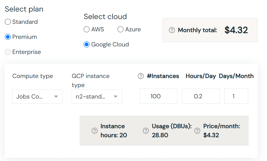
• Databricks Compute: Running two notebooks for 4 hours on a job cluster costs $4.32 at $0.15 per DBU.

  
  

  

  
  

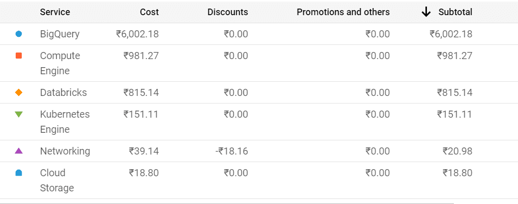
• GCP Infrastructure: The underlying Kubernetes cluster and Virtual Machine(VM) Instances adds an additional $13.44.

  
  

  

Expected Annual Cost Savings

We assume that the tasks will run 365 days on both BigQuery and Databricks

          Platform               Calculation                    Annual Cost 
        ————————————————————————————————————————————————————————————————————
          BigQuery          (Data Loading : $20 +
        (On-Demand)         Queries : $7 ) * 365                  $9855  
        ————————————————————————————————————————————————————————————————————
          Databricks        (Compute : $4.32 + 
                         GCP Infrastructure : $13.44)             $6482 
                                 * 365 
        ————————————————————————————————————————————————————————————————————

Based on this simplified example, Databricks has the potential to save you a whopping 34% annually.

Remember, this is a simplified comparison. Here's what to consider before making your final decision:

• Data Storage Needs: How much data will you be storing and how often will you access it?

• Workload Complexity: Are your jobs simple queries or complex data transformations?

• Scalability Requirements: Do your needs fluctuate, or is your workload consistent?

Databricks might be your champion for cost savings, especially for compute-intensive tasks. But with its flexibility and potential for savings, Databricks could be the MVP for your data adventures!

Conclusion

The most cost-effective platform hinges on your specific workload:

1. Databricks for: (Give Databricks the edge here!):

   • Workloads with complex transformations or data engineering tasks.

   • The potential for significant cost savings through right-sizing DBU usage and leveraging spot instances.

     
     

2. BigQuery (On-Demand) for:

   • Unpredictable workloads with smaller, frequent queries.